Cartooning Images
May 20, 2018
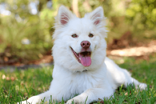
In this post, I will demonstrate a simple application of variational methods in computer vision. We receive an RGB image of any size as input and want to give it a cartoonish looking style.
Variational methods?
In these approaches, one typically specifies a probability distribution over the hidden variables that are conditioned upon observed variables and optionally a prior distribution on the hidden variables. This is the model definition phase, then one either performs an inference to uncover properties of the distribution or seeks a particular solution. A solution is just an instantiation of hidden variables, i.e. an assignment of values. Often, one looks for the mode of the distribution. A typical workflow in this approach is as follows:
- Specify a probabilistic model that captures the problem well
- Convert it to an error/energy function
- Optimize the error function
Throughout this post we use the following notation
- \(A \in \mathbb{R}^{k \times n}\)
- \(A_{i:}\) is i-th row of A
- \(A_{:i}\) is i-th column of A
Model
For our problem, we will follow the above-mentioned steps as well. In fact, we are going to skip the first step and directly specify a convex error function and optimize it using projected gradient descent. In our case, the observed variables are the RGB values of the pixels and the hidden variables are the cartoonified RGB values of the pixels. Typically, error functions consist of multiple terms enforcing different characteristics for the hidden variables. For this problem, we will use two terms, a data term and a regularizer term.
Data Term
This term usually measures a dissimilarity between the input/observed-variables and the output/hidden-variables, thus enforcing a similarity between. In our case, it implies that the cartoonified image should to look similar to the input image. We define it as the following:
\(E_{Data} = \text{tr}(U^T F) = u_{11}f_{11} + u_{12}f_{12} + \ldots + u_{kn}f_{kn}\)
- \(\text{tr}(\cdot)\) is trace operator
- \(U \in \mathbb{R}^{k \times n}\)
- \(F \in \mathbb{R}^{k \times n}\)
- n is the number of pixels in input image
What do U, F and k represent?
According to our formulation, every pixel in the cartoonified image is one of \(k\) colors. Here \(k\) is a rather small number (e.g. 5) because in general cartoon images contain only a handful of colors. Let \(C\) be set of cartoon colors. What colors are reasonable to have in \(U\)? There is no absolute way to answer this, though it makes sense to put some dominant colors from the input image. We will get back to this later.
F Matrix
Once we decide on \(C\), we can construct the matrix \(F\) where \(F_{ij}\) measures dissimilarity between the color of the j-th pixel and the i-th color in \(C\). For a demonstration let's say we picked \(C = \{\text{red}, \text{green}, \text{blue}, \text{white}, \text{black}\}\) and constructed \(F\) accordingly. The first row of \(F\) will be a measure of distance of the original image from the color red, the second row of \(F\) for green, so on and so forth. See the following figure for a visualization of each row of \(F\) for this situation.


U Matrix
In our problem, \(U\) matrix is the hidden variables we are going to optimize for. It is not a cartoon image though, but a voting table. In our formulation, every pixel will vote for colors in \(C\) to be converted to. For instance, if \(C\) contains 3 colors and pixel 1 votes:
- 20% for \(c_1\) (color 1 in \(C\))
- 70% for \(c_2\) (color 2 in \(C\))
- 10% for \(c_3\) (color 3 in \(C\))
then we pick \(C_2\) to be the color for pixel 1 in the cartoonified image. Therefore, once we decide on \(U\), we construct the cartoonified image with the "elected" colors for each pixel. Note that we have the following constraints for \(U\):
- \(0 \leq U_{ij} \leq 1\), for \(1 \leq i \leq k\) and \(1 \leq j \leq n\)
- \(\|U_{:i}\|_1 = 1\), for \(1 \leq i \leq n\)
Where \(\|\cdot\|\) is the L1-norm and \(U_{:i}\) is the i-th column of U.
Regularizing Term
This term usually measures the variance or extremity of output/hidden-variables, thus enforcing a smoothness. In our case, it implies that the cartoonified image should consist of large intact regions. We define it as the following:
- \(\|\cdot\|\) is the L2-norm operator
- \(D \in \mathbb{R}^{2n \times n}\) is a gradient computing matrix both in x-direction and y-direction
- \(\alpha\) is a hyper-parameter adjusting the relative importance of smoothness
Construction of matrix D is beyond the scope of this post, therefore, we will assume that it is available to us.
Approach
We will optimize the error function using gradient descent. The catch here is that we do not want to violate the constraints laid out for columns of U. They must stay in the set of k-dimensional simplex. Therefore after update step, we use a sub-procedure described in [1] to project each row back to k-dimensional simplex. The details of this algorithm are again beyond the intention of this post.
Gradient Calculation
Data term
The gradient due to this term is very straightforward:
Regularizer term
Before computing this, let's declare two well known derivating rules when we deal with vectors and matrices.
| Variable | Gradient |
|---|---|
| \(x \in \mathbb{R}^n\) | \(\frac{d(\|x\|)}{dx} = \frac{x^T}{\|x\|}\) |
| \(x \in \mathbb{R}^n, A \in \mathbb{R}^{k \times n}\) | \(\frac{d(Ax)}{dx} = A\) |
Let's unfold the summation in the regularizer term and compute the gradient. After applying the chain rule and the derivative rules above, we get:
Combining the gradient of the data-term and the regularizer term, we get the complete gradient:
The following code computes the gradient as described:
Implementation
There is one thing that we did not elaborate on: selection of color set. How do we decide which colors to use in the cartoon image? Again there is no single answer to this. Some approaches could be:
- Hand-pick \(C\)
- Cluster the colors in the image and pick \(k\) of them
In my implementation, I picked \(C\) as the cluster centers resulting from the output of k-means algorithm on image colors. The colors are as following when \(k = 5\):

The MATLAB script to perform projected gradient descent is as follows:
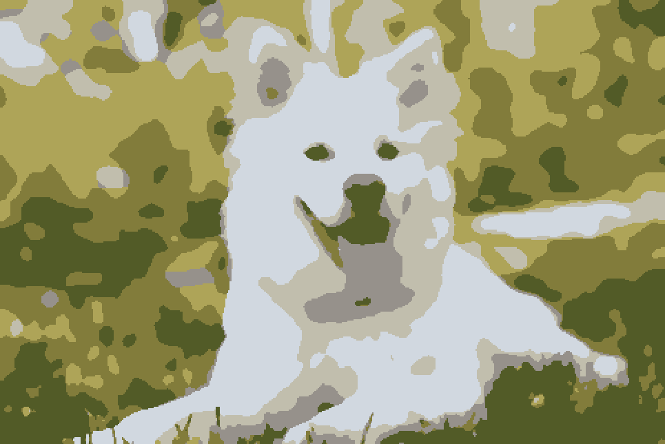
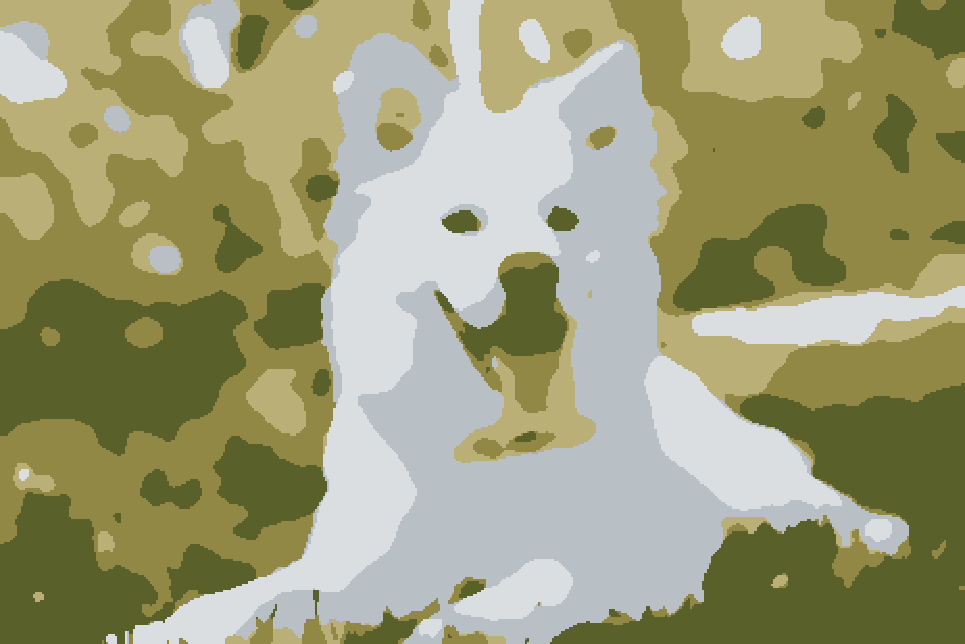
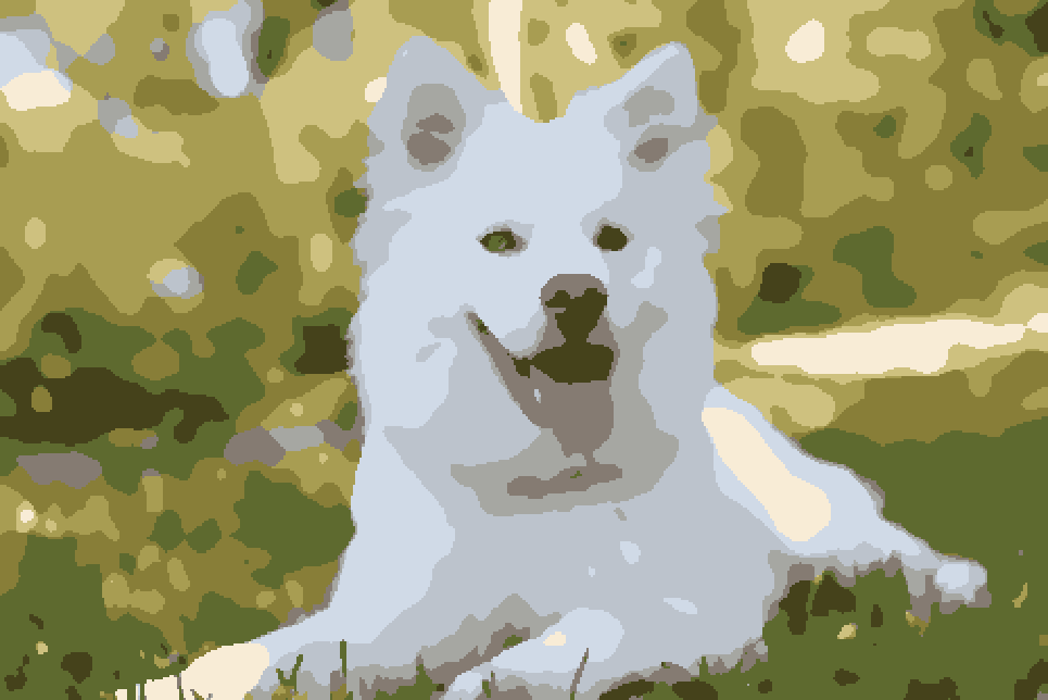
See an example evolution of the dog image starting from a random initialization:
Results of some experiments with different selections of hyper-parameters:
References
[1] Chen, Yunmei, and Xiaojing Ye. "Projection onto a simplex." arXiv preprint arXiv:1101.6081 (2011).